Image Colourisation

You might have already used some AI Picture Colourizer software (such as Vance AI). Such software is being used for the reconstruction of old B&W photographs or films of historical and cultural significance or of sentimental value to the user of the application software. But how does this software work? Is it really possible to recover all lost colour information?

B&W

Reconstructed

Coloured

Unfortunately, most algorithms can only make informed guesses about the colour content of an image and frequently fail in the complete absence of any colour information. Using Vance AI to reproduce the colour content of those B&W peppers, we see that many colours are not identified correctly. There have been multiple cases of image colourising that provoked anxiety about the authenticity of photography in the digital era as covered in this article.

A simple remedy to this may be to simplify the problem by adding some colour information to the image. Perhaps the colour of certain objects in the image are known or can be easily guessed by the user of such software. This simplifies the problem and increases our confidence in the reconstructed colourized image.

B&W+colour dots

Reconstructed

Coloured

Consider a rectangular image with $k$ horizontal pixels and $l$ vertical pixels. The task is to find the RGB values for every pixel. Hence, the algorithm needs to return three vectors $(R,G,B)$ of length $m=kl$, with each component corresponding to a pixel. The greyscale information of the image is also a vector if length $m$ and it is given. All values are in the interval $[0,1]$.

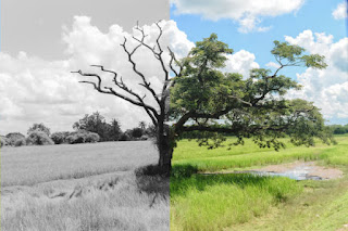
Images consist of two forms of information; luma and chrominance. Luma represents the brightness/luminosity of an image corresponding to the greyscale information, while chrominance conveys pure colour information after getting rid of the luma. In our problem, we are given all the luma/greyscale information but little chrominance information and we try to reconstruct the rest of it.

Original image (left) decomposed to luma (centre) and chrominance (right).

The brightness of a pixel depends linearly on the RGB values of that pixel, but the coefficients of the three colours are not the same. Green is a much brighter colour than blue, so an empirical formula (Rec 601 encoding) for the brightness/greyscale is that it comes 60% from green intensity, 30% from red intensity and only 10% from the blue intensity.

In certain few pixels of the image we are also given their colour (chrominance) content. In other words, the RGB values are given for a few $n\ll m$ pixels in the image. Consider an uncoloured pixel; the task is to colour it by adding the colour contribution from each of the n coloured pixels. This colour contribution to uncoloured pixel $x$ from coloured pixel $y$ is represented by the impact factor or kernel function $k(x,y)$.  If two pixels are close to each other and have similar greyscale values, it is very likely that they share similar RGB values, so we want the impact factor of $y$ on $x$ to be high when the distance of the pixels and their greyscale difference is small and low when either of these assumptions fail. We formulate this impact factor as

$$k(x,y)=\varphi \left(\frac{d(x,y)}{{\sigma }_1}\right)\varphi \left(\frac{|\gamma (x)-\gamma (y){|}^p}{{\sigma }_2}\right),\text{where}$$

·       $\gamma (t)$ is the greyscale value of pixel $t$,

·       $d(x,y)$ represents the distance of pixel $x$ and $y$ in the image,

·       and $\varphi$ is a decaying radial basis function, such as the Gaussian radial function or some compactly supported radial function (e.g. Wendland), with

·       hyperparameter ${\sigma }_1,{\sigma }_2$ being the decay scales and $0<p<1$.

Different Kernel functions

The colour information given in these points radially “spreads” to the rest of the image, colouring the uncoloured pixels. You can imagine the coloured pixels as light sources, radiating their colour information with decaying intensity and regulated by jumps in greyscale information which may indicate a change of colour.

Since there are n coloured points $\{y_1,\dots ,y_n\}$, the reconstructed RGB values of the uncoloured pixel x is a linear combination of the impact factors $k(x,y_i)$. The coefficients of that linear functions differ for each of the three colours and need to be found through optimization. The cost function that we try to minimize is the squared residual of the reconstructed colour values of $y_1,\dots ,y_n$ with the addition of a regularization term that penalizes the colour intensity in order to avoid overfitting and exceeding the maximum colour values. This turns out to be a linear problem with respect to the coefficients, so we may use a standard linear solver. If compact support radial function is used, the resulting matrix of the linear problem is sparse and symmetric, which can speed up calculations.

But how do we choose hyperparameters ${\sigma }_1,{\sigma }_2,p,\delta$? We start by guessing the values and proceed with training the model on a given image with known colorized content. The hyperparameters should minimize the sum of RGB residual values (reconstructed values found with those hyperparameters minus true values).

Optimal hyperparameters were found for $140$ images which can be found here. Those images have been manually classified as either ‘cartoon-like’ or as ‘artistic’ depending on how sharp the changes in greyscale were, with cartoon images having sharp borders.

Artistic Images

    Cartoon Images

For Wendland's compact support function as kernel, which strongly outperformed the Gaussian kernel function, the optimal values for ${\sigma }_1$ and $\delta$ are typically around $0.3$ and $1\mathrm{e}-4$ respectively. Meanwhile, the optimal values of ${\sigma }_2$ and $p$ take a range of values across different figures and are strongly dependent on each other.

Optimal hyperparameters ${\sigma }_2$ and $p$ in log scale.

Since there is a linear relationship between $\log {\sigma }_2$ and $\log p$, the user would only be required to give only one value; perhaps through a slider for ${\sigma }_2$. Even simpler than that, they can specify whether their image looks more like a cartoon figure or a more fluid/artistic figure, with $(p,{\sigma }_2)$ for cartoon and artistic images being $(0.6,0.2)$ and $(0.8,0.6)$ respectively. For those recommended values, the critical greyscale difference beyond which the impact factor vanishes is $7\mathrm{\%}$ of the I scale for cartoon images and $42\mathrm{\%}$ for artistic. This is not surprising, since even relatively small changes in the greyscale content of cartoon images could indicate that a border has been crossed between completely different colour regions.